Project Definition Using devices such as Jawbone Up, Nike FuelBand, and Fitbit it is now possible to collect a large amount of data about personal activity relatively inexpensively. These type of devices are part of the quantified self movement – a group of enthusiasts who take measurements about themselves regularly to improve their health, to find patterns in their behavior, or because they are tech geeks. One thing that people regularly do is quantify how much of a particular activity they do, but they rarely quantify how well they do it. In this project, your goal will be to use data from accelerometers on the belt, forearm, arm, and dumbell of 6 participants. They were asked to perform barbell lifts correctly and incorrectly in 5 different ways. More information is available from the website here: http://groupware.les.inf.puc-rio.br/har (see the section on the Weight Lifting Exercise Dataset).
- Given by Coursera Course Coordinator

Step 1 : Include R Packages

library(caret);

library(AppliedPredictiveModeling);

library(randomForest);

library(knitr);

library(rpart);

library(rpart.plot);

library(rattle);

library(corrplot)

Step 2 : Loading training and testing datasets

Train <- "http://d396qusza40orc.cloudfront.net/predmachlearn/pml-training.csv"

Test <- "http://d396qusza40orc.cloudfront.net/predmachlearn/pml-testing.csv"

training <- read.csv(url(Train))

testing <- read.csv(url(Test))

Step 3 : Create Data Partition

inTrain <- createDataPartition(training$classe, p=0.7, list=FALSE)

TrainSet <- training[inTrain, ]

TestSet <- training[-inTrain, ]

Step 4 : Preprocess the data to drop zero and NAN values

NonZV <- nearZeroVar(TrainSet)

TrainSet <- TrainSet[, -NonZV]

TestSet <- TestSet[, -NonZV]

NA_ALL <- sapply(TrainSet, function(x) mean(is.na(x))) > 0.95

TrainSet <- TrainSet[, NA_ALL==FALSE]

TestSet <- TestSet[, NA_ALL==FALSE]

Dropping the first five columns from the training and testing dataset>

TrainSet <- TrainSet[, -(1:5)]

TestSet <- TestSet[, -(1:5)]

Step 5 : Random Forest to train and predict model

set.seed(12345)

controlRF <- trainControl(method="cv", number=3, verboseIter=FALSE)

modRF <- train(classe ~ ., data=TrainSet, method="rf", + trControl=controlRF)

modRF$finalModel

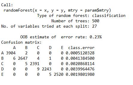
predictRF <- predict(modFitRandForest, newdata=TestSet)

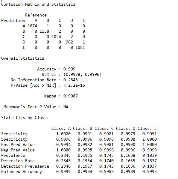
To print the confusion matrix we need to factor both the predicRF and TestSet for equal levels. So here I have called the as.factor function within the confusionMatrix () functions.

Statistics_RF <- confusionMatrix(predictRF, as.factor(TestSet$classe))

Statistics_RF

Step 6 : Decision Tree to train and predict model

set.seed(12345)

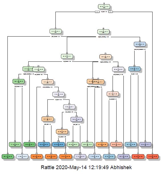
modDT <- rpart(classe ~ ., data=TrainSet, method="class")

fancyRpartPlot(modDT)

predictDecTree <- predict(modDT, newdata=TestSet, type="class")

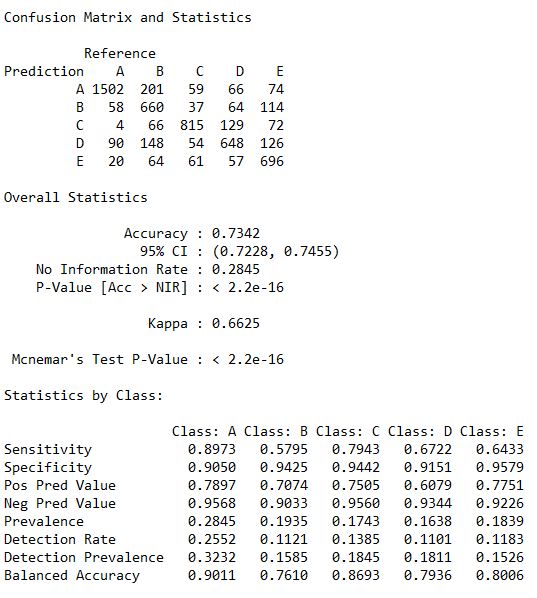
To print the confusion matrix we need to factor both the predicDecTree and TestSet for equal levels. So here I have called the as.factor function within the confusionMatrix () functions.

Staestics_DT <- confusionMatrix(predictDecTree, as.factor(TestSet$classe))

Statistics_DT

Step 7 : GBM to train and predict model

set.seed(12345)

controlGBM <- trainControl(method = "repeatedcv", number = 5, repeats = 1)

modGBM <- train(classe ~ ., data=TrainSet, method = "gbm", + trControl = controlGBM, verbose = FALSE)

modGBM$finalModel

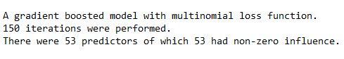
predictGBM <- predict(modGBM, newdata=TestSet)

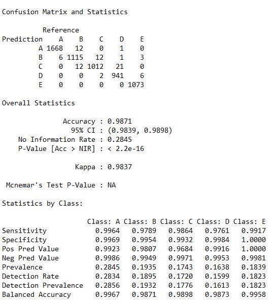
To print the confusion matrix we need to factor both the predicGBM and TestSet for equal levels. So here I have called the as.factor function within the confusionMatrix () functions.

Statestics_GBM <- confusionMatrix(predictGBM, as.factor(TestSet$classe))

Statistics_GBM

Step 8 : Final Result

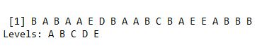
predictTEST <- predict(modRF, newdata=testing)

predictTEST

I. RandomForest (RF) : Accuracy : 0.9963

II. Decision Tree (DT) : Accuracy : 0.7368

III.Gradient Boosting Model (GBM) : 0.9871

Step 7 : Conclusion

Thus the best working model is Random Forest only.bold>